mAP(mean Average Precision) 指标笔记

mAP是目标识别中常用的指标，下面介绍其具体计算方法，包含这几个部分：召回率、精度、准确率、PR曲线、AUC。

参考：Object-Detection-Metrics

召回率、精度、准确率

这三个参数是传统二分类问题中所涉及的，用于评价二分类模型的性能。而目标识别问题也可以视为一个二分类问题，我们将图像中所有预测出的识别框都视为正例，其他所有的可能预测框都为负例，所以数据集中负例的数量将是无穷，但是没事，我们的指标中不会用到负例。

假设我们有一个二分类模型，对于数据集中的每个样本，模型给出一个对应的预测，我们将预测的结果分为以下四个类别：

1. TP/FP (True/False Positive)：正确/错误 预测为正例的样本数目。
2. TN/FN (True/False Negative)：正确/错误 预测为负例的样本数目。

我们不难发现这两个性质：$TP+FN=:N_{pos}$ 为数据集中全部正例数目，$TN+FP=:N_{neg}$ 为数据集中全部负例数目，整个数据集大小为 $N_{pos} + N_{neg} =: N$。

如下定义召回率(Recall)，精度(Precision)和准确率(Accuracy)：

$$\begin{cases} R = \dfrac{TP}{TP+FN} = \dfrac{TP}{N_{p}},\text{整个数据集中全部正例预测准确的比例}\\ \\ P = \dfrac{TP}{TP+FP},\text{全部预测为正例中正确的比例}\\ \\ A = \dfrac{TP+TN}{N},\text{整个数据集中预测正确的比例} \end{cases}$$

目标识别问题

从二分类问题上看

在目标识别问题中，由于模型给出的预测框都可以认为是正例，所以 $TN=FN=0$。在该问题下精度和准确率相同，即 $A=P=\dfrac{TP}{TP+FP}$，召回率重新定义为 $R=\dfrac{TP}{N_{box}}$，其中 $N_{box}$ 表示整个数据集中真实框的数目（和二分类中的 $N_{pos}$ 相同）。

正例的确定方法

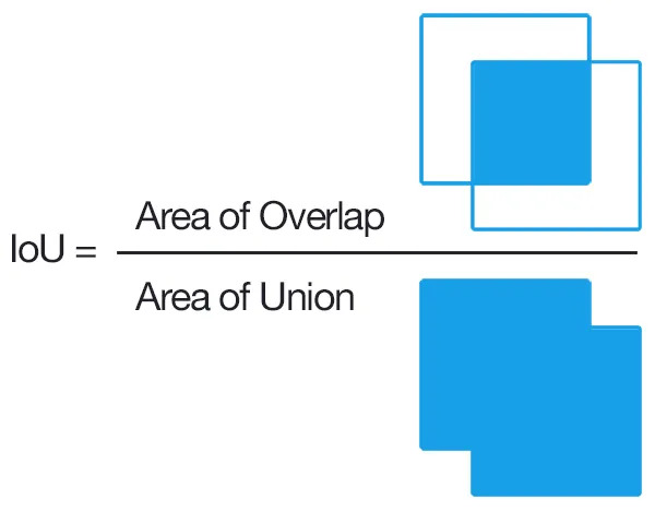
在目标识别问题中，如果确定一个识别框是正确的呢？我们需要引入两个边界框的IOU（Intersection over Union）概念，IOU定义为两个框的相交面积除以两个框并起来的面积，如下所示：

我们通过如下两步判断一个置信度为 $conf$ 的预测框 $b^{pred}$ 是否是预测正确的，假设该图像中包含 $n$ 个检测框：

1. 在数据集中找到与 $b^{pred}$ 有最大IOU的真实框，记为 $b^{gt}$，当IOU大于给定阈值 $\alpha$ 时，进行下一步。
2. 在当前图像预测出的 $m$ 个检测框中，若 $\forall b_i^{pred}, (i=1,\cdots,m)$ 满足 $conf_i > conf$，都 $\exists b_{j}^{gt}, (j=1,\cdots,n)$ 使得 $IOU_{b_i^{pred}}^{b_j^{gt}} > IOU_{b_i^{pred}}^{b^{gt}}$（没有另一个更大置信度的预测框和当前预测框抢真实框）

如果当前预测框 $(b^{pred}, conf)$ 满足上述两个条件，则属于TP（正确预测的正例），否则为FP（错误预测的正例）。

PR曲线

我们将全部预测框按照置信度从大到小排序，逐一在坐标系上描点，对于描的第 $i$ 个点，考虑预测框中前 $i$ 大置信度的框所计算得到的精度 $P_i$、召回率 $R_i$，在坐标系上绘制点 $(R_i,P_i)$，最后将点按照绘制顺序依次连接，即为PR曲线。不难发现，$R_i$ 单调递增。

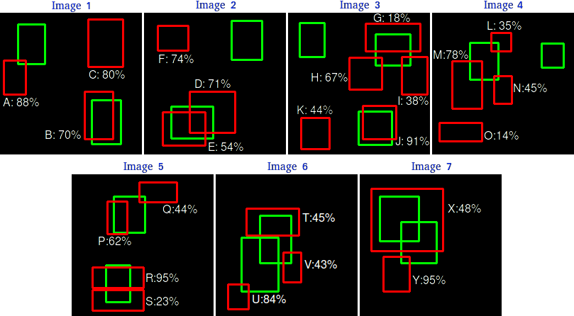
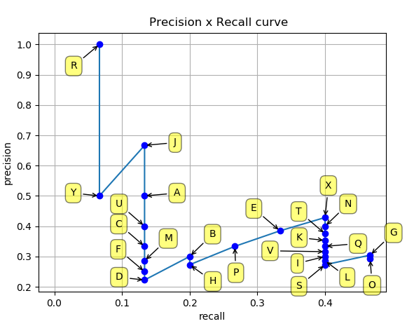
如上图所示，左图将预测框编号为从A~Y，按照置信度从大到小排序后，逐一计算累计精度和召回率，绘制在右图中并连接，即可得到PR曲线。

AP及mAP

AP指标（Average Percision）就是对精度的平均，通常用PR曲线下面积AUC（Area Under Curve）来表示。

mAP指标（mean Average Percision）就是基于类别对AP值进行平均，假设边界框总共 $C$ 个类别，对于第 $c$ 个类别，我们可以在固定的IOU阈值 $\alpha$ 下，计算出对应的AP值，记为 $AP_c$，则mAP定义为

$$mAP = \frac{1}{C}\sum_{c=1}^CAP_c$$

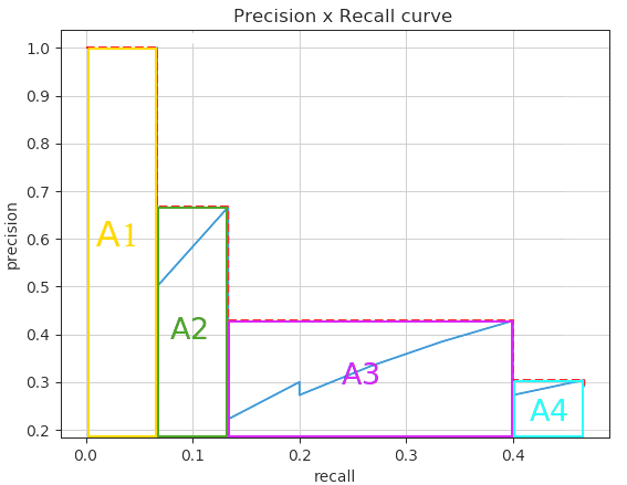
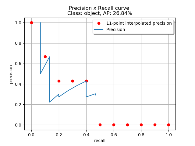
如下图所示，左图表示全部的AUC曲线下面积，右图表示使用11个插值点计算得到的估计值。（值得注意的是，曲线下面积是每个点的右侧最高值进行估计得到的，所以算出的结果比真实曲线下面积更大一些）

---

最后再总结一下，对于一个目标识别模型，给定一个数据集和一个IOU阈值 $\alpha\in(0,1)$ （用于判断预测框是否预测正确），我们就对每个类别 $c=1,\cdots, C$ 求出 $AP_c$，然后平均求得 $mAP$ 值。

COCO mAP

那么我们是不是还要问 $\alpha$ 取值是多少？不难看出，当 $\alpha$ 趋近于 $1$ 时，当预测框准确预测时的要求更高，通常我们取 $10$ 种不同的 $\alpha$，分别为 $0.5,0.55,0.6,\cdots,0.9,0.95$，步长为 $0.05$，设由阈值 $\alpha$ 算出的mAP记为 $mAP@\alpha$ 或 $mAP@(100\alpha)$，则COCO数据集的mAP评测指标为

$$mAP@[50:95:5] := \frac{1}{10}\sum_{i=0}^{9}mAP@(50+5i)$$

常用的mAP预测指标还有 $mAP@50$ 和 $mAP@75$。

代码实现

1. 用NMS对模型预测出的重复框进行筛选。
2. 对每张图中所有预测框，分别计算10种不同IOU阈值下，每个预测框是否为正确的正例（TP, True Positive）
3. 将所有图片的所有预测框以及在不同IOU阈值下计算的TP值进行合并。
4. 对每个类别 $c$，统计数据集中属于类别 $c$ 的真实框数目 $N_c$，计算不同置信度下的累计TP，FP值。
5. 对每个类别 $c$，分别求出对应累计置信度下的精度、召回率（此处可以求出 $P@50$ 和 $R@50$ 分别表示在所有置信度大于 $0.1$ 的预测框，在 $0.5$ IOU阈值下的精度召回率）。
6. 最后对10个不同IOU阈值求出离散的PR曲线，用101点插值（COCO）或11点插值（PASCAL VOC），对曲线下面积AUC进行估计，从而得到 $AP_c@\alpha,(c=1,\cdots,C,\alpha=50,55\cdots,90,95)$，从而求出 $mAP@\alpha,mAP@[50:95:5]$。

计算AP值的核心代码如下，参考 YOLOv4官方代码：

def ap_per_class(tp, conf, pcls, tcls):
  """
  Compute AP for each class in `np.unique(tcls)`.

  Args:
    tp: True positive of the predicted bounding boxes. [shape=(N,10) or (N,1)]
    conf: Confidence of the predicted bounding boxes. [shape=(N,)]
    pcls: Class label of the predicted bounding boxes. [shape=(N,)]
    tcls: Class label of the target bounding boxes. [shape=(M,)]
  
  Return:
    p: Precision for each class with confidence bigger than 0.1. [shape=(Nc,tp.shape[1])]
    r: Recall for each class with confidence bigger than 0.1. [shape=(Nc,tp.shape[1])]
    ap: Average precision for each class with different iou thresholds. [shape=(Nc,tp.shape[1])]
    f1: F1 coef for each class with confidence bigger than 0.1. [shape=(Nc,)]
    ucls: Class labels after being uniqued. [shape=(Nc,)]
  """
  sort_i = np.argsort(-conf)
  tp, conf, pcls = tp[sort_i], conf[sort_i], pcls[sort_i]
  ucls = np.unique(tcls)
  shape = (len(ucls), tp.shape[1])
  ap, p, r = np.zeros(shape), np.zeros(shape), np.zeros(shape)
  pr_score = 0.1
  for i, cls in enumerate(ucls):
    idx = pcls == cls
    # number of predict and target boxes with class `cls`
    n_p, n_t = idx.sum(), (tcls==cls).sum()
    if n_p == 0: continue
    fpc = (1-tp[idx]).cumsum(0)  # cumulate false precision
    tpc = tp[idx].cumsum(0)  # cumulate true precision
    recall = tpc / n_t
    r[i] = np.interp(-pr_score, -conf[idx], recall[:,0])  # conf[idx] decrease
    precision = tpc / (tpc + fpc)
    p[i] = np.interp(-pr_score, -conf[idx], precision[:,0])
    for j in range(tp.shape[1]):
      ap[i,j] = compute_ap(recall[:,j], precision[:,j])
  f1 = 2 * p * r / (p + r + 1e-5)
  return p, r, ap, f1, ucls.astype(np.int32)

def compute_ap(recall, precision, mode='interp'):
  """
  Compute the average precision (AP) by the area under the curve (AUC) \
  of the Recall x Precision curve.

  Args:
    recall: Recall of the predicted bounding boxes. [shape=(N,)]
    precision: Precision of the predicted bounding boxes. [shape=(N,)]
    mode: The mode of calculating the area. ['continue' or 'interp']
      interp: 101-point interpolation (COCO: https://cocodataset.org/#detection-eval).
      continue: all the point where `recall` changes.
  
  Return:
    ap: The area under the `recall` x `precision` curve.
  """
  # Add sentinel values to begin and end
  r = np.concatenate([(0.0,), recall, (min(recall[-1]+1e-5, 1.0),)])
  p = np.concatenate([(0.0,), precision, (0.0,)])
  # Compute the precision envelope
  p = np.flip(np.maximum.accumulate(np.flip(p)))

  if mode == 'interp':
    x = np.linspace(0, 1, 101)
    ap = np.trapz(np.interp(x, r, p), x)
  elif mode == 'continue':
    i = np.where(r[1:]!=r[:-1])[0]
    ap = np.sum((r[i+1] - r[i]) * p[i])  # p[i] == p[i+1]
  return ap