《机器学习实战》第二章 端到端的机器学习项目
最新更新于: 2024年5月24日上午11点17分
端到端的机器学习项目实例
《机器学习实战:基于Scikit-Learn,Keras和TensorFlow》中第二章内容,英文代码可参考github - handson-ml2/02_end_to_end_machine_learning_project.ipynb
下面内容对应的Jupyter Notebook代码位于github:2.end_to_end_machine_learning_project.ipynb
数据集预处理
数据集下载位置:https://raw.githubusercontent.com/ageron/handson-ml2/master/datasets/housing/housing.tgz
将 housing.tgz 文件放到 ./datasets/housing 下.
import numpy as np
import pandas as pd
import matplotlib.pyplot as plt
from pathlib import Path
import tarfile

DATASETS_ROOT = r"https://raw.githubusercontent.com/ageron/handson-ml2/master/datasets"
HOUSING_PATH = Path.cwd().joinpath('./datasets/housing')
HOUSING_URL = DATASETS_ROOT + "/housing/housing.tgz"
print('数据集路径:', HOUSING_PATH)

def fetch_housing_data(url=HOUSING_URL, path=HOUSING_PATH):
    path.mkdir(parents=True, exist_ok=True)  # 创建本地目录
    save_path = path.joinpath('housing.tgz')  # 保存路径
    housing_tgz = tarfile.open(save_path)
    housing_tgz.extractall(path=path)
    housing_tgz.close()

fetch_housing_data()
数据集路径: D:\yy\DeepLearning\ml-scikit-keras-tf2\datasets\housing
def load_housing_data(path=HOUSING_PATH):
    csv_path = path.joinpath('housing.csv')
    return pd.read_csv(csv_path)

df = load_housing_data()df.head()| longitude | latitude | housing_median_age | total_rooms | total_bedrooms | population | households | median_income | median_house_value | ocean_proximity | |
|---|---|---|---|---|---|---|---|---|---|---|
| 0 | -122.23 | 37.88 | 41.0 | 880.0 | 129.0 | 322.0 | 126.0 | 8.3252 | 452600.0 | NEAR BAY |
| 1 | -122.22 | 37.86 | 21.0 | 7099.0 | 1106.0 | 2401.0 | 1138.0 | 8.3014 | 358500.0 | NEAR BAY |
| 2 | -122.24 | 37.85 | 52.0 | 1467.0 | 190.0 | 496.0 | 177.0 | 7.2574 | 352100.0 | NEAR BAY |
| 3 | -122.25 | 37.85 | 52.0 | 1274.0 | 235.0 | 558.0 | 219.0 | 5.6431 | 341300.0 | NEAR BAY |
| 4 | -122.25 | 37.85 | 52.0 | 1627.0 | 280.0 | 565.0 | 259.0 | 3.8462 | 342200.0 | NEAR BAY |
df.info()<class 'pandas.core.frame.DataFrame'>
RangeIndex: 20640 entries, 0 to 20639
Data columns (total 10 columns):
# Column Non-Null Count Dtype
--- ------ -------------- -----
0 longitude 20640 non-null float64
1 latitude 20640 non-null float64
2 housing_median_age 20640 non-null float64
3 total_rooms 20640 non-null float64
4 total_bedrooms 20433 non-null float64
5 population 20640 non-null float64
6 households 20640 non-null float64
7 median_income 20640 non-null float64
8 median_house_value 20640 non-null float64
9 ocean_proximity 20640 non-null object
dtypes: float64(9), object(1)
memory usage: 1.6+ MB
df['ocean_proximity'].value_counts()<1H OCEAN 9136
INLAND 6551
NEAR OCEAN 2658
NEAR BAY 2290
ISLAND 5
Name: ocean_proximity, dtype: int64
df.describe()| longitude | latitude | housing_median_age | total_rooms | total_bedrooms | population | households | median_income | median_house_value | |
|---|---|---|---|---|---|---|---|---|---|
| count | 20640.000000 | 20640.000000 | 20640.000000 | 20640.000000 | 20433.000000 | 20640.000000 | 20640.000000 | 20640.000000 | 20640.000000 |
| mean | -119.569704 | 35.631861 | 28.639486 | 2635.763081 | 537.870553 | 1425.476744 | 499.539680 | 3.870671 | 206855.816909 |
| std | 2.003532 | 2.135952 | 12.585558 | 2181.615252 | 421.385070 | 1132.462122 | 382.329753 | 1.899822 | 115395.615874 |
| min | -124.350000 | 32.540000 | 1.000000 | 2.000000 | 1.000000 | 3.000000 | 1.000000 | 0.499900 | 14999.000000 |
| 25% | -121.800000 | 33.930000 | 18.000000 | 1447.750000 | 296.000000 | 787.000000 | 280.000000 | 2.563400 | 119600.000000 |
| 50% | -118.490000 | 34.260000 | 29.000000 | 2127.000000 | 435.000000 | 1166.000000 | 409.000000 | 3.534800 | 179700.000000 |
| 75% | -118.010000 | 37.710000 | 37.000000 | 3148.000000 | 647.000000 | 1725.000000 | 605.000000 | 4.743250 | 264725.000000 |
| max | -114.310000 | 41.950000 | 52.000000 | 39320.000000 | 6445.000000 | 35682.000000 | 6082.000000 | 15.000100 | 500001.000000 |
df.hist(bins=50, figsize=(18, 12))
plt.show()
np.random.seed(42)  # 固定初始随机种子
def split_train_test(df, test_ratio):
    shuffled_indices = np.random.permutation(len(df))
    test_size = int(len(df) * test_ratio)
    test_indices = shuffled_indices[:test_size]
    train_indices = shuffled_indices[test_size:]
    return df.iloc[train_indices], df.iloc[test_indices]

train_df, test_df = split_train_test(df, 0.2)
print('训练集大小:', len(train_df), '测试集大小:', len(test_df))
训练集大小: 16512 测试集大小: 4128
两种划分训练集与测试集的方法
-
使用上述方式,确定随机种子后,可以保证对于同一数据集的随机结果保持相同,但缺点是如果加入新的数据,划分出的训练集与测试集内容可能完全不同.
-
利用每个样本的Hash值,作为划分标准,一个样本的Hash值需要是该样本的唯一标识符,例如:“索引”,“房产的经纬度”
# 利用Hash值进行划分
from zlib import crc32

def test_check(identifier, test_ratio):
    return crc32(np.int64(identifier)) & 0xffffffff < test_ratio * 2**32  # 左侧为使用crc32计算出的Hash值

def split_train_test_by_hash(df, test_ratio, id_column):
    ids = df[id_column]
    is_test = ids.apply(lambda id_: test_check(id_, test_ratio))
    return df.loc[~is_test], df.loc[is_test]

df_idx = df.reset_index()
train, test = split_train_test_by_hash(df_idx, 0.2, 'index')
print('训练集大小:', len(train_df), '测试集大小:', len(test_df))
训练集大小: 16512 测试集大小: 4128
使用Scikit-Learn中的方法对数据进行划分
-
设定随机种子进行均匀划分,
train_test_split(df, test_size=0.2, random_state=42):df为数据集,test_size为测试集比例,random_state为随机种子. -
分层划分数据集,由于测试集需要代表整个数据集的整体信息,首先对数据特征进行层划分,在每一层中,我们希望都要有足够的信息来表示这种类别,表示该层的重要程度.
首先利用 pd.cut() 对层进行划分,例如划分为 这样 段.
再使用Scikit中的api函数实例化划分模型 split=StratifiedShuffleSplit(n_splits=1, test_size=0.2, random_state=42):n_splits 表示划分的总数据集个数,test_size 为测试集占比,random_state 表示随机种子.
最后通过迭代方式生成训练集与测试集:train_idx, test_idx = next(split.split(df, df['income_cat']))(由于只生成一个数据集,所以可以直接用next获取第一个迭代结果)
from sklearn.model_selection import train_test_split

train, test = train_test_split(df, test_size=0.2, random_state=42)
print('训练集大小:', len(train_df), '测试集大小:', len(test_df))
训练集大小: 16512 测试集大小: 4128
df['income_cat'] = pd.cut(df['median_income'], bins=[0., 1.5, 3., 4.5, 6., np.inf], labels=[1,2,3,4,5])
df['income_cat'].hist()
plt.show()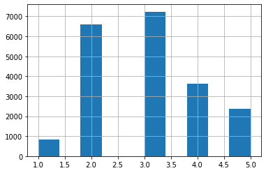
from sklearn.model_selection import StratifiedShuffleSplit

split = StratifiedShuffleSplit(n_splits=1, test_size=0.2, random_state=42)
# for train_idx, test_idx in split.split(df, df['income_cat']):
train_idx, test_idx = next(split.split(df, df['income_cat']))
strat_train = df.loc[train_idx]
strat_test = df.loc[test_idx]

strat_income_ratio = strat_test['income_cat'].value_counts() / len(strat_test)
base_income_ratio = df['income_cat'].value_counts() / len(df)
test_income_cate = pd.cut(test['median_income'], bins=[0., 1.5, 3., 4.5, 6., np.inf], labels=[1,2,3,4,5])
random_income_ratio = test_income_cate.value_counts() / len(test)
def calc_error(base, x):
return (x - base) / base * 100
diff_test_sample = pd.concat([base_income_ratio, strat_income_ratio, random_income_ratio,
calc_error(base_income_ratio, strat_income_ratio),
calc_error(base_income_ratio, random_income_ratio)], axis=1)
diff_test_sample.columns = ['Overall', 'Stratified', 'Random', 'Strated error %', 'Random error %']
diff_test_sample = diff_test_sample.sort_index()
diff_test_sample| Overall | Stratified | Random | Strated error % | Random error % | |
|---|---|---|---|---|---|
| 1 | 0.039826 | 0.039971 | 0.040213 | 0.364964 | 0.973236 |
| 2 | 0.318847 | 0.318798 | 0.324370 | -0.015195 | 1.732260 |
| 3 | 0.350581 | 0.350533 | 0.358527 | -0.013820 | 2.266446 |
| 4 | 0.176308 | 0.176357 | 0.167393 | 0.027480 | -5.056334 |
| 5 | 0.114438 | 0.114341 | 0.109496 | -0.084674 | -4.318374 |
# 删除income_cat该列
for ds in (strat_train, strat_test):
    ds.drop('income_cat', axis=1, inplace=True)
数据集可视化
config = {
    "font.family": 'serif', # 衬线字体
    "figure.figsize": (6, 6),  # 图像大小
    "font.size": 16, # 字号大小
    "font.serif": ['SimSun'], # 宋体
    "mathtext.fontset": 'stix', # 渲染数学公式字体
    'axes.unicode_minus': False # 显示负号
}
plt.rcParams.update(config)

df = strat_train.copy()
df.plot(kind='scatter', x='longitude', y='latitude', alpha=0.1, xlabel='经度', ylabel='纬度', figsize=(6, 6))
plt.show()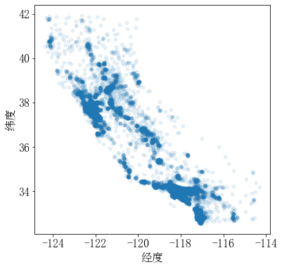
import matplotlib as mpl
ax = df.plot(kind='scatter', x='longitude', y='latitude', alpha=0.4,
        s=df['population']/100, label='人口数', figsize=(10, 7),
        c='median_house_value', cmap='jet', colorbar=False,
        xlabel='经度', ylabel='纬度')
ax.figure.colorbar(plt.cm.ScalarMappable(
    norm=mpl.colors.Normalize(vmin=df['median_house_value'].min(), vmax=df['median_house_value'].max()), cmap='jet'),
    label='房价中位数', alpha=0.4)
plt.legend()
plt.show()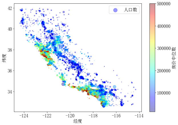
数据相关性
# Pearson's correlation coefficient
corr_matrix = df.corr()
corr_matrix['median_house_value'].sort_values(ascending=False)
median_house_value 1.000000
median_income 0.687151
total_rooms 0.135140
housing_median_age 0.114146
households 0.064590
total_bedrooms 0.047781
population -0.026882
longitude -0.047466
latitude -0.142673
Name: median_house_value, dtype: float64
from pandas.plotting import scatter_matrix

attributes = ['median_house_value', 'median_income', 'total_rooms', 'housing_median_age']
scatter_matrix(df[attributes], figsize=(15, 10))
plt.show()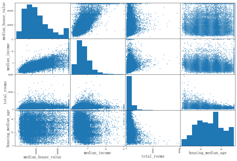
数据清理
df_x = strat_train.drop('median_house_value', axis=1)
df_y = strat_train['median_house_value'].copy()
df_x.info()
<class 'pandas.core.frame.DataFrame'>
Int64Index: 16512 entries, 12655 to 19773
Data columns (total 9 columns):
# Column Non-Null Count Dtype
--- ------ -------------- -----
0 longitude 16512 non-null float64
1 latitude 16512 non-null float64
2 housing_median_age 16512 non-null float64
3 total_rooms 16512 non-null float64
4 total_bedrooms 16354 non-null float64
5 population 16512 non-null float64
6 households 16512 non-null float64
7 median_income 16512 non-null float64
8 ocean_proximity 16512 non-null object
dtypes: float64(8), object(1)
memory usage: 1.3+ MB
df_x[df_x['total_bedrooms'].isna()]| longitude | latitude | housing_median_age | total_rooms | total_bedrooms | population | households | median_income | ocean_proximity | |
|---|---|---|---|---|---|---|---|---|---|
| 1606 | -122.08 | 37.88 | 26.0 | 2947.0 | NaN | 825.0 | 626.0 | 2.9330 | NEAR BAY |
| 10915 | -117.87 | 33.73 | 45.0 | 2264.0 | NaN | 1970.0 | 499.0 | 3.4193 | <1H OCEAN |
| 19150 | -122.70 | 38.35 | 14.0 | 2313.0 | NaN | 954.0 | 397.0 | 3.7813 | <1H OCEAN |
| 4186 | -118.23 | 34.13 | 48.0 | 1308.0 | NaN | 835.0 | 294.0 | 4.2891 | <1H OCEAN |
| 16885 | -122.40 | 37.58 | 26.0 | 3281.0 | NaN | 1145.0 | 480.0 | 6.3580 | NEAR OCEAN |
| ... | ... | ... | ... | ... | ... | ... | ... | ... | ... |
| 1350 | -121.95 | 38.03 | 5.0 | 5526.0 | NaN | 3207.0 | 1012.0 | 4.0767 | INLAND |
| 4691 | -118.37 | 34.07 | 50.0 | 2519.0 | NaN | 1117.0 | 516.0 | 4.3667 | <1H OCEAN |
| 9149 | -118.50 | 34.46 | 17.0 | 10267.0 | NaN | 4956.0 | 1483.0 | 5.5061 | <1H OCEAN |
| 16757 | -122.48 | 37.70 | 33.0 | 4492.0 | NaN | 3477.0 | 1537.0 | 3.0546 | NEAR OCEAN |
| 13336 | -117.67 | 34.04 | 13.0 | 1543.0 | NaN | 776.0 | 358.0 | 3.0598 | INLAND |
158 rows × 9 columns
df_x.fillna(0).loc[1606]longitude -122.08
latitude 37.88
housing_median_age 26.0
total_rooms 2947.0
total_bedrooms 0.0
population 825.0
households 626.0
median_income 2.933
ocean_proximity NEAR BAY
Name: 1606, dtype: object
# 使用Scikit-Learn中的填补方式
from sklearn.impute import SimpleImputer
imputer = SimpleImputer(strategy='median')  # 利用每列的中位数进行填补
df_num = df_x.drop('ocean_proximity', axis=1)
train_x = imputer.fit_transform(df_num)
from sklearn.preprocessing import OrdinalEncoder
ordinal_encoder = OrdinalEncoder()
df_cat_encoded = ordinal_encoder.fit_transform(df_cat)
df_cat_encoded[:10]array([[1.],
[4.],
[1.],
[4.],
[0.],
[3.],
[0.],
[0.],
[0.],
[0.]])
from sklearn.preprocessing import OneHotEncoder
onehot_encoder = OneHotEncoder()
df_cat_onehot = onehot_encoder.fit_transform(df_cat)
df_cat_onehot[:10].toarray()
array([[0., 1., 0., 0., 0.],
[0., 0., 0., 0., 1.],
[0., 1., 0., 0., 0.],
[0., 0., 0., 0., 1.],
[1., 0., 0., 0., 0.],
[0., 0., 0., 1., 0.],
[1., 0., 0., 0., 0.],
[1., 0., 0., 0., 0.],
[1., 0., 0., 0., 0.],
[1., 0., 0., 0., 0.]])
自定义转化器
通过该转化器可以为特征(Character)增加新的属性(Attribute):
-
每户平均所用房间数:
rooms_per_households. -
每户平均人口数:
population_per_households. -
每间房的平均卧室数:
bedrooms_per_rooms. (可选是否添加)
所需列的索引编号分别有 total_rooms, total_bedrooms, population, households
from sklearn.base import BaseEstimator, TransformerMixin

class CombinedAttributersAdder(BaseEstimator, TransformerMixin):
    def __init__(self, idxs, add_bedrooms_per_rooms=True):
        self.idxs = idxs
        self.add_bedrooms_per_rooms = add_bedrooms_per_rooms
    def fit(self, X, y=None):
        return self
    def transform(self, X):
        rooms_per_households = (X[:, self.idxs['total_rooms']] / X[:, self.idxs['households']]).reshape([-1,1])
        population_per_households = (X[:, self.idxs['population']] / X[:, self.idxs['households']]).reshape([-1,1])
        ret = [X, rooms_per_households, population_per_households]
        if self.add_bedrooms_per_rooms:
            ret.append((X[:, self.idxs['total_bedrooms']] / X[:, self.idxs['total_rooms']]).reshape([-1,1]))
        return np.concatenate(ret, axis=1)

idxs = dict([(col, i) for i, col in enumerate(df_x.columns)])
attr_adder = CombinedAttributersAdder(idxs, add_bedrooms_per_rooms=False)
df_extra_attribs = attr_adder.fit_transform(df_x.values)
df_extra_attribs.shape
(16512, 11)
attr_adder.set_params(add_bedrooms_per_rooms=False)
attr_adder.get_params()
{'add_bedrooms_per_rooms': False,
'idxs': {'longitude': 0,
'latitude': 1,
'housing_median_age': 2,
'total_rooms': 3,
'total_bedrooms': 4,
'population': 5,
'households': 6,
'median_income': 7,
'ocean_proximity': 8}}
特征缩放
-
归一化
MinMaxScaler,将数据集减去最小值后除以最大值,X = (X - np.min(X)) / np.max(X). -
标准化
StandardScaler,将数据集减去均值后除以标准差,X = (X - np.mean(X)) / np.std(X).
from sklearn.preprocessing import StandardScaler
from sklearn.preprocessing import MinMaxScaler
std_scaler = StandardScaler()
mm_scaler = MinMaxScaler()
X = np.array(df_x[['housing_median_age']])
scale1 = std_scaler.fit_transform(X)
scale2 = mm_scaler.fit_transform(X)
X1 = (X - np.mean(X)) / np.std(X)
X2 = (X - np.min(X)) / np.max(X)
转换流水线
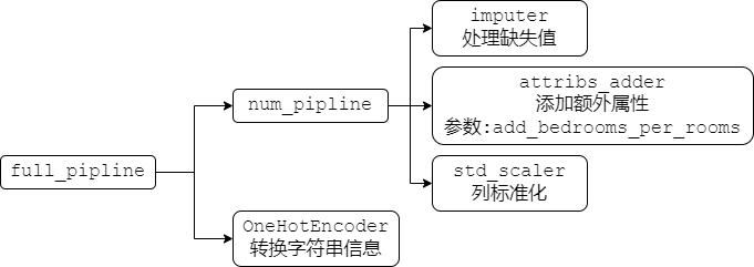
在Scikit-Learn中 Pipline 是由一系列的转换器进行的堆叠(也就是必须要有 fit_transform() 函数),而堆叠的最后一个只需是一个估计器(也就是可以只有 fit() 函数),最后流水线也具有最后一个估计器的功能,如果最后一个估计器有 transform() 函数,那么流水线也有 fit_transform() 函数,如果最后一个估计器有 predict() 函数,那么流水线也具有 fit_predict() 函数.
Pipline 的构造函数包含一个元组列表,每个元组包含 (名称, 转化器),第一个属性为转化器的名称,命名自定义(不包含双下划线,不能重复),第二个属性为转化器构造函数
from sklearn.pipeline import Pipeline

num_pipeline = Pipeline([
    ('imputer', SimpleImputer(strategy="median")),
    ('attribs_adder', CombinedAttributersAdder(idxs, add_bedrooms_per_rooms=True)),
    ('std_scaler', StandardScaler()),
])
df_num_tr = num_pipeline.fit_transform(df_num)
df_num_tr.shape
(16512, 11)
对不同列分别进行转换
由于原数据集中既有数字特征,也有文本特征,所以需要分别做预处理,sklearn.compose.ColumnTransformer 可以很好的完成这项操作. 它可以非常好的适配 DataFrame 数据类型,通过列索引找到需要处理的列,最后逇返回值,会根据最终矩阵的稠密度来判断是否使用稀疏矩阵还是密集矩阵(矩阵密度定义为非零值的占比,默认阈值为 sparse_threshold=0.3)
构造函数中,需要一个元组列表,每个元组包含 名称, 转化器, 列索引列表,名称同 Pipline 的要求(自定义,不重复,无双下划线),列索引列表可以直接为 DataFrame 中的列名.
from sklearn.compose import ColumnTransformer

# 从分层抽样后的训练数据中划分出特征与标签
df_x = strat_train.drop('median_house_value', axis=1)
df_num = df_x.drop('ocean_proximity', axis=1)  # 划分出纯数字特征,便于预处理
train_y = np.array(strat_train['median_house_value'])  # 注意不要破坏原始数据集

num_attribs = list(df_num)  # numeral
cat_attribs = ['ocean_proximity']  # category

full_pipline = ColumnTransformer([
    ('num', num_pipeline, num_attribs),  # 将数字使用之前的pipline进行转化
    ('cat', OneHotEncoder(), cat_attribs),  # 将字符串转化为one-hot类别
])

train_x = full_pipline.fit_transform(df_x)
选择与训练模型
这里我们将尝试三种基本机器学习模型,并选择其中较好的模型进一步微调:
-
线性回归模型.
-
决策树模型.
-
随机森林模型.
# 线性回归
from sklearn.linear_model import LinearRegression

lin_reg = LinearRegression()
lin_reg.fit(train_x, train_y)  # 模型估计

x = train_x[:5]
y = train_y[:5]
print("Predictions:", lin_reg.predict(x))  # 预测结果
print("Labels", list(y))
Predictions: [ 85657.90192014 305492.60737488 152056.46122456 186095.70946094
244550.67966089]
Labels [72100.0, 279600.0, 82700.0, 112500.0, 238300.0]
from sklearn.metrics import mean_squared_error
lin_mse = mean_squared_error(train_y, lin_reg.predict(train_x))
lin_rmse = np.sqrt(lin_mse)
print("Line RMSE:", lin_rmse)  # 欠拟合
Line RMSE: 68627.87390018745
# 决策树
from sklearn.tree import DecisionTreeRegressor

tree_reg = DecisionTreeRegressor()
tree_reg.fit(train_x, train_y)

tree_mse = mean_squared_error(train_y, tree_reg.predict(train_x))
tree_rmse = np.sqrt(tree_mse)
print("Tree RMSE:", tree_rmse)  # 严重过拟合
Tree RMSE: 0.0
交叉验证
一种简单的方法是使用 train_test_split 将训练集进一步划分为较小的训练集和验证集,然后使用较小的数据集进行训练,并在验证集上进行评估.
另一种方便的做法是使用Scikit-Learn中的K-折交叉验证功能 sklearn.model_selection.cross_val_score,假设 ,则具体做法是将训练集随机划分为10个不同的子集,每个子集称为一个折叠,对模型进行10次训练与评估——每次选取1个折叠作为验证集,剩余9个折叠作为训练集,返回一个包含10次评分的数组,评分规则可以在 scoring 属性中设定.
from sklearn.model_selection import cross_val_score
from sklearn.metrics import make_scorer

tree_scores = cross_val_score(tree_reg, train_x, train_y, scoring=make_scorer(mean_squared_error), cv=5)
lin_scores = cross_val_score(lin_reg, train_x, train_y, scoring=make_scorer(mean_squared_error), cv=5)
def display_scores(scores):
print("得分:", scores)
print("均值:", scores.mean())
print("标准差:", scores.std())
print('决策树:')
display_scores(np.sqrt(tree_scores))
print('\n线性回归:')
display_scores(np.sqrt(lin_scores)) # 从均值可以看出决策树比线性回归还差决策树:
得分: [69044.77910565 70786.57350426 68989.97289114 74120.47872383
70840.03725076]
均值: 70756.36829512753
标准差: 1864.1267179081194
线性回归:
得分: [68076.63768302 67881.16711321 69712.97514343 71266.9225777
68390.25096271]
均值: 69065.59069601327
标准差: 1272.9445955637493
# 随机森林模型
from sklearn.ensemble import RandomForestRegressor

forest_reg = RandomForestRegressor()
forest_reg.fit(train_x, train_y)
forest_scores = cross_val_score(forest_reg, train_x, train_y, scoring=make_scorer(mean_squared_error), cv=5)print('随机森林:')
display_scores(np.sqrt(forest_scores)) # 均值最小,说明该模型效果不错随机森林:
得分: [49944.24394028 50069.54102601 49720.76735777 51561.67277575
51410.4086245 ]
均值: 50541.32674486087
标准差: 780.8734448089192
# 模型保存
import joblib

joblib.dump(forest_reg, "forest.pkl")
model_loaded = joblib.load("forest.pkl")

model_loaded.set_params(verbose=0)
model_loaded.predict(train_x[:5])  # 尝试简单预测
array([ 72910., 293380., 81403., 124556., 228456.])
模型微调
可以从交叉验证结果看出随机森林效果不错,下面对其参数进行进一步微调.
网格搜索
通过Scikit-Learn的 sklearn.model_selection.GridSearchCV 可以方便的尝试模型不同给定的参数组合,其会在不同的参数组合下进行交叉验证,所以也有 cv 参数设置,交叉验证的打分结果默认为越大越好,所以是负的均方误差 neg_mean_squared_error.
from sklearn.model_selection import GridSearchCV
from sklearn.ensemble import RandomForestRegressor

params_grid = [
    {'n_estimators': [3, 10, 30], 'max_features': [2, 4, 6, 8]},
    {'bootstrap': [False], 'n_estimators': [3, 10], 'max_features': [2, 3, 4]},
]
forest_reg = RandomForestRegressor(random_state=42)

grid_search = GridSearchCV(forest_reg, params_grid, cv=5, scoring='neg_mean_squared_error', return_train_score=True)
grid_search.fit(train_x, train_y)
# 输出最好的组合及得分
print("参数组合:", grid_search.best_params_)
print("得分:", np.sqrt(-grid_search.best_score_))参数组合: {'max_features': 8, 'n_estimators': 30}
得分: 49898.98913455217
# 输出不同参数对应的均值RMSE
cvres = grid_search.cv_results_
for mean_score, params in zip(cvres['mean_test_score'], cvres['params']):
    print(np.sqrt(-mean_score), params)
63895.161577951665 {'max_features': 2, 'n_estimators': 3}
54916.32386349543 {'max_features': 2, 'n_estimators': 10}
52885.86715332332 {'max_features': 2, 'n_estimators': 30}
60075.3680329983 {'max_features': 4, 'n_estimators': 3}
52495.01284985185 {'max_features': 4, 'n_estimators': 10}
50187.24324926565 {'max_features': 4, 'n_estimators': 30}
58064.73529982314 {'max_features': 6, 'n_estimators': 3}
51519.32062366315 {'max_features': 6, 'n_estimators': 10}
49969.80441627874 {'max_features': 6, 'n_estimators': 30}
58895.824998155826 {'max_features': 8, 'n_estimators': 3}
52459.79624724529 {'max_features': 8, 'n_estimators': 10}
49898.98913455217 {'max_features': 8, 'n_estimators': 30}
62381.765106921855 {'bootstrap': False, 'max_features': 2, 'n_estimators': 3}
54476.57050944266 {'bootstrap': False, 'max_features': 2, 'n_estimators': 10}
59974.60028085155 {'bootstrap': False, 'max_features': 3, 'n_estimators': 3}
52754.5632813202 {'bootstrap': False, 'max_features': 3, 'n_estimators': 10}
57831.136061214274 {'bootstrap': False, 'max_features': 4, 'n_estimators': 3}
51278.37877140253 {'bootstrap': False, 'max_features': 4, 'n_estimators': 10}
pd.DataFrame(grid_search.cv_results_)| mean_fit_time | std_fit_time | mean_score_time | std_score_time | param_max_features | param_n_estimators | param_bootstrap | params | split0_test_score | split1_test_score | ... | mean_test_score | std_test_score | rank_test_score | split0_train_score | split1_train_score | split2_train_score | split3_train_score | split4_train_score | mean_train_score | std_train_score | |
|---|---|---|---|---|---|---|---|---|---|---|---|---|---|---|---|---|---|---|---|---|---|
| 0 | 0.056342 | 0.003779 | 0.003243 | 0.000397 | 2 | 3 | NaN | {'max_features': 2, 'n_estimators': 3} | -4.119912e+09 | -3.723465e+09 | ... | -4.082592e+09 | 1.867375e+08 | 18 | -1.155630e+09 | -1.089726e+09 | -1.153843e+09 | -1.118149e+09 | -1.093446e+09 | -1.122159e+09 | 2.834288e+07 |
| 1 | 0.195027 | 0.017347 | 0.009637 | 0.001599 | 2 | 10 | NaN | {'max_features': 2, 'n_estimators': 10} | -2.973521e+09 | -2.810319e+09 | ... | -3.015803e+09 | 1.139808e+08 | 11 | -5.982947e+08 | -5.904781e+08 | -6.123850e+08 | -5.727681e+08 | -5.905210e+08 | -5.928894e+08 | 1.284978e+07 |
| 2 | 0.549724 | 0.007784 | 0.022255 | 0.000432 | 2 | 30 | NaN | {'max_features': 2, 'n_estimators': 30} | -2.801229e+09 | -2.671474e+09 | ... | -2.796915e+09 | 7.980892e+07 | 9 | -4.412567e+08 | -4.326398e+08 | -4.553722e+08 | -4.320746e+08 | -4.311606e+08 | -4.385008e+08 | 9.184397e+06 |
| 3 | 0.085986 | 0.001792 | 0.002960 | 0.000096 | 4 | 3 | NaN | {'max_features': 4, 'n_estimators': 3} | -3.528743e+09 | -3.490303e+09 | ... | -3.609050e+09 | 1.375683e+08 | 16 | -9.782368e+08 | -9.806455e+08 | -1.003780e+09 | -1.016515e+09 | -1.011270e+09 | -9.980896e+08 | 1.577372e+07 |
| 4 | 0.283107 | 0.012133 | 0.008094 | 0.000168 | 4 | 10 | NaN | {'max_features': 4, 'n_estimators': 10} | -2.742620e+09 | -2.609311e+09 | ... | -2.755726e+09 | 1.182604e+08 | 7 | -5.063215e+08 | -5.257983e+08 | -5.081984e+08 | -5.174405e+08 | -5.282066e+08 | -5.171931e+08 | 8.882622e+06 |
| 5 | 0.846614 | 0.018781 | 0.025807 | 0.006609 | 4 | 30 | NaN | {'max_features': 4, 'n_estimators': 30} | -2.522176e+09 | -2.440241e+09 | ... | -2.518759e+09 | 8.488084e+07 | 3 | -3.776568e+08 | -3.902106e+08 | -3.885042e+08 | -3.830866e+08 | -3.894779e+08 | -3.857872e+08 | 4.774229e+06 |
| 6 | 0.109496 | 0.001429 | 0.003194 | 0.000403 | 6 | 3 | NaN | {'max_features': 6, 'n_estimators': 3} | -3.362127e+09 | -3.311863e+09 | ... | -3.371513e+09 | 1.378086e+08 | 13 | -8.909397e+08 | -9.583733e+08 | -9.000201e+08 | -8.964731e+08 | -9.151927e+08 | -9.121998e+08 | 2.444837e+07 |
| 7 | 0.371871 | 0.006231 | 0.008252 | 0.000400 | 6 | 10 | NaN | {'max_features': 6, 'n_estimators': 10} | -2.622099e+09 | -2.669655e+09 | ... | -2.654240e+09 | 6.967978e+07 | 5 | -4.939906e+08 | -5.145996e+08 | -5.023512e+08 | -4.959467e+08 | -5.147087e+08 | -5.043194e+08 | 8.880106e+06 |
| 8 | 1.130365 | 0.010059 | 0.022360 | 0.000711 | 6 | 30 | NaN | {'max_features': 6, 'n_estimators': 30} | -2.446142e+09 | -2.446594e+09 | ... | -2.496981e+09 | 7.357046e+07 | 2 | -3.760968e+08 | -3.876636e+08 | -3.875307e+08 | -3.760938e+08 | -3.861056e+08 | -3.826981e+08 | 5.418747e+06 |
| 9 | 0.143730 | 0.002764 | 0.003008 | 0.000005 | 8 | 3 | NaN | {'max_features': 8, 'n_estimators': 3} | -3.590333e+09 | -3.232664e+09 | ... | -3.468718e+09 | 1.293758e+08 | 14 | -9.505012e+08 | -9.166119e+08 | -9.033910e+08 | -9.070642e+08 | -9.459386e+08 | -9.247014e+08 | 1.973471e+07 |
| 10 | 0.479244 | 0.002045 | 0.008288 | 0.000386 | 8 | 10 | NaN | {'max_features': 8, 'n_estimators': 10} | -2.721311e+09 | -2.675886e+09 | ... | -2.752030e+09 | 6.258030e+07 | 6 | -4.998373e+08 | -4.997970e+08 | -5.099880e+08 | -5.047868e+08 | -5.348043e+08 | -5.098427e+08 | 1.303601e+07 |
| 11 | 1.444280 | 0.008099 | 0.022597 | 0.000362 | 8 | 30 | NaN | {'max_features': 8, 'n_estimators': 30} | -2.492636e+09 | -2.444818e+09 | ... | -2.489909e+09 | 7.086483e+07 | 1 | -3.801679e+08 | -3.832972e+08 | -3.823818e+08 | -3.778452e+08 | -3.817589e+08 | -3.810902e+08 | 1.916605e+06 |
| 12 | 0.086494 | 0.001798 | 0.003198 | 0.000396 | 2 | 3 | False | {'bootstrap': False, 'max_features': 2, 'n_est... | -4.020842e+09 | -3.951861e+09 | ... | -3.891485e+09 | 8.648595e+07 | 17 | -0.000000e+00 | -4.306828e+01 | -1.051392e+04 | -0.000000e+00 | -0.000000e+00 | -2.111398e+03 | 4.201294e+03 |
| 13 | 0.284451 | 0.004976 | 0.009399 | 0.000489 | 2 | 10 | False | {'bootstrap': False, 'max_features': 2, 'n_est... | -2.901352e+09 | -3.036875e+09 | ... | -2.967697e+09 | 4.582448e+07 | 10 | -0.000000e+00 | -3.876145e+00 | -9.462528e+02 | -0.000000e+00 | -0.000000e+00 | -1.900258e+02 | 3.781165e+02 |
| 14 | 0.112028 | 0.007602 | 0.004233 | 0.001024 | 3 | 3 | False | {'bootstrap': False, 'max_features': 3, 'n_est... | -3.687132e+09 | -3.446245e+09 | ... | -3.596953e+09 | 8.011960e+07 | 15 | -0.000000e+00 | -0.000000e+00 | -0.000000e+00 | -0.000000e+00 | -0.000000e+00 | 0.000000e+00 | 0.000000e+00 |
| 15 | 0.364553 | 0.003523 | 0.009679 | 0.000402 | 3 | 10 | False | {'bootstrap': False, 'max_features': 3, 'n_est... | -2.837028e+09 | -2.619558e+09 | ... | -2.783044e+09 | 8.862580e+07 | 8 | -0.000000e+00 | -0.000000e+00 | -0.000000e+00 | -0.000000e+00 | -0.000000e+00 | 0.000000e+00 | 0.000000e+00 |
| 16 | 0.136975 | 0.001282 | 0.003008 | 0.000004 | 4 | 3 | False | {'bootstrap': False, 'max_features': 4, 'n_est... | -3.549428e+09 | -3.318176e+09 | ... | -3.344440e+09 | 1.099355e+08 | 12 | -0.000000e+00 | -0.000000e+00 | -0.000000e+00 | -0.000000e+00 | -0.000000e+00 | 0.000000e+00 | 0.000000e+00 |
| 17 | 0.447112 | 0.003923 | 0.009294 | 0.000389 | 4 | 10 | False | {'bootstrap': False, 'max_features': 4, 'n_est... | -2.692499e+09 | -2.542704e+09 | ... | -2.629472e+09 | 8.510266e+07 | 4 | -0.000000e+00 | -0.000000e+00 | -0.000000e+00 | -0.000000e+00 | -0.000000e+00 | 0.000000e+00 | 0.000000e+00 |
18 rows × 23 columns
grid_search.cv_results_.keys()dict_keys(['mean_fit_time', 'std_fit_time', 'mean_score_time', 'std_score_time', 'param_max_features', 'param_n_estimators', 'param_bootstrap', 'params', 'split0_test_score', 'split1_test_score', 'split2_test_score', 'split3_test_score', 'split4_test_score', 'mean_test_score', 'std_test_score', 'rank_test_score', 'split0_train_score', 'split1_train_score', 'split2_train_score', 'split3_train_score', 'split4_train_score', 'mean_train_score', 'std_train_score'])
from sklearn.model_selection import RandomizedSearchCV
from scipy.stats import randint

params_distrib = [
    {'n_estimators': randint(28, 33), 'max_features': randint(7, 10)},
]
forest_reg = RandomForestRegressor(random_state=42)

rand_search = RandomizedSearchCV(forest_reg, params_distrib, cv=5, n_iter=20, random_state=42,
                                 scoring='neg_mean_squared_error', return_train_score=True)
rand_search.fit(train_x, train_y)
# 输出最好的组合及得分,可以看出随机组合的得分比网格搜索的结果更好
print("参数组合:", rand_search.best_params_)
print("得分:", np.sqrt(-rand_search.best_score_))参数组合: {'max_features': 8, 'n_estimators': 32}
得分: 49842.263664875936
# 尝试过的组合及对应的打分
cvres = rand_search.cv_results_
for mean_score, params in zip(cvres['mean_test_score'], cvres['params']):
    print(np.sqrt(-mean_score), params)
50073.941984726036 {'max_features': 9, 'n_estimators': 31}
49928.56733204831 {'max_features': 7, 'n_estimators': 30}
49855.054296768314 {'max_features': 7, 'n_estimators': 32}
50154.159979801916 {'max_features': 9, 'n_estimators': 29}
50118.217225106 {'max_features': 9, 'n_estimators': 30}
50076.27434408333 {'max_features': 9, 'n_estimators': 32}
50076.27434408333 {'max_features': 9, 'n_estimators': 32}
49882.90700266577 {'max_features': 8, 'n_estimators': 31}
49911.07348226599 {'max_features': 8, 'n_estimators': 29}
49947.86413574509 {'max_features': 7, 'n_estimators': 28}
49842.263664875936 {'max_features': 8, 'n_estimators': 32}
49947.86413574509 {'max_features': 7, 'n_estimators': 28}
50118.217225106 {'max_features': 9, 'n_estimators': 30}
50154.159979801916 {'max_features': 9, 'n_estimators': 29}
50118.217225106 {'max_features': 9, 'n_estimators': 30}
50073.941984726036 {'max_features': 9, 'n_estimators': 31}
49928.56733204831 {'max_features': 7, 'n_estimators': 30}
49928.56733204831 {'max_features': 7, 'n_estimators': 30}
50076.27434408333 {'max_features': 9, 'n_estimators': 32}
49904.569413113204 {'max_features': 7, 'n_estimators': 29}
# 随机森林模型有每种类别的重要性分数
feature_importances = rand_search.best_estimator_.feature_importances_
# 进一步我们可以获得每种类别的重要度排名
extra_attribs = ['rooms_per_households', 'popultion_per_households', 'bedrooms_per_rooms']  # 额外加入的属性
cat_encoder = full_pipline.named_transformers_['cat']
cat_attribs = list(cat_encoder.categories_[0])  # 字符串列表
attributes = list(df_num) + extra_attribs + cat_attribs
sorted(zip(feature_importances, attributes), reverse=True)
[(0.38172022914549825, 'median_income'),
(0.165994178010966, 'INLAND'),
(0.10653004837910676, 'popultion_per_households'),
(0.06894855994908974, 'longitude'),
(0.059534576077903516, 'latitude'),
(0.05392562234554215, 'rooms_per_households'),
(0.04722669031431806, 'bedrooms_per_rooms'),
(0.043182846603246804, 'housing_median_age'),
(0.015983911178773656, 'population'),
(0.015450335997150988, 'total_bedrooms'),
(0.01527186966684709, 'total_rooms'),
(0.014934070980648344, 'households'),
(0.006547710175385619, '<1H OCEAN'),
(0.0031214750700245385, 'NEAR OCEAN'),
(0.0015469548512138229, 'NEAR BAY'),
(8.092125428472885e-05, 'ISLAND')]
测试集上评估
model = rand_search.best_estimator_

df_x = strat_test.drop('median_house_value', axis=1)
test_y = np.array(strat_test['median_house_value'])

test_x = full_pipline.transform(df_x)  # 注意使用transform而不是fit_transform
test_pred = model.predict(test_x)

rmse = mean_squared_error(test_y, test_pred, squared=False)
rmse
47886.90979155171
# 计算泛化误差置信度为0.95的置信区间用来评估模型效果
from scipy import stats

confidence = 0.95
squared_errors = (test_y - test_pred) ** 2
np.sqrt(stats.t.interval(confidence, len(squared_errors)-1, loc=squared_errors.mean(), scale=stats.sem(squared_errors)))
array([45902.05283165, 49792.7083478 ])
练习题
- 第一个练习题是使用SVM进行预测,看作者的代码结果效果并不如随机森林好,所以跳过.
- 用
RandomizedSearchCV替换GridSearchCV,已经在上面对随机森林实验过了,效果不错.
3. 在流水线中添加一个转化器用于筛选重要信息
现有的流水线包括:
期望在 full_pipline 后面再加入 TopFeatureSelector 根据特征的重要性排序进行选择最高的特征值,具有属性 k 表示选取前 k 重要的属性值.
注意!!
由于对OneHotEncoder也在每次折叠数据中,由于包含 Island 的数据仅有5个,所以部分折叠数据集可能完全没有 Island,就会导致OneHotEncoder不会对其进行编码,导致列数目减少一个,所以一定要判断列数(其实正确做法应该是在数据读入进来时就将字符串数据进行OneHot表示,就不会有这些问题了)
arg_sorted = np.argsort(feature_importances)[::-1]
class TopFeatureSelector(BaseEstimator, TransformerMixin):
    def __init__(self, k=5):
        self.k = k
    def fit(self, x, y=None):
        return self
    def transform(self, x):
        now_arg = arg_sorted.copy()
        if x.shape[1] == 15:  # 如果输入数据中没有ISLAND列,将最后5列索引向前移
            now_arg[now_arg > 13] -= 1
        return x[:, now_arg[:self.k]]

preparer_and_selector_pipline = Pipeline([
    ('preparer', full_pipline),
    ('feature_selector', TopFeatureSelector()),
])

train_x_selected = preparer_and_selector.fit_transform(df_x)  # 经过重要度选择后的列
preparer_and_selector_pipline  # 显示完整预处理流水线
4. 创建一个覆盖完整的数据准备和最终预测的流水线
在 preparer_and_selector_pipline 的基础上加上预测器即可
df_train_x = strat_train.drop('median_house_value', axis=1)
complete_pipline = Pipeline([
    ('preparer_and_seletor', preparer_and_selector_pipline),
    ('model', RandomForestRegressor(**rand_search.best_params_)),
])
complete_pipline.fit(df_train_x, train_y)
# 测试集上进行计算得分
df_test_x = strat_test.drop('median_house_value', axis=1)
test_pred = complete_pipline.predict(df_test_x)
mean_squared_error(test_y, test_pred, squared=False)49064.16896575968
5. 使用GridSearchCV自动探寻超参数
基于 complete_pipline 和双下划线 __ 可以修改内部估计器的超参数. 预计修改的超参数:
preparer_and_seletor__feature_selector__k:选择前k重要的特征,preparer_and_seletor__preparer__num__imputer__strategy:三种填补缺失值策略median, mean, most_frequent.
params_grid = [  # 总共尝试个数3x2x3=18
    {'preparer_and_seletor__preparer__cat__handle_unknown': ['ignore'],  # 关键,onehot编码可能在transform中见到fit中未见到的值,所以会报错,一定要加入ignore来保证输出结果正确
     'preparer_and_seletor__feature_selector__k': [5, 10, 15, 16],
     'preparer_and_seletor__preparer__num__imputer__strategy': ['median', 'mean', 'most_frequent']
    },
]

grid_search = GridSearchCV(complete_pipline, params_grid, cv=5, scoring='neg_mean_squared_error', verbose=2, error_score='raise')
grid_search.fit(df_train_x, train_y)print('得分:', np.sqrt(-grid_search.best_score_))
print('参数:', grid_search.best_params_)得分: 49934.92197039834
参数: {'preparer_and_seletor__feature_selector__k': 15, 'preparer_and_seletor__preparer__cat__handle_unknown': 'ignore', 'preparer_and_seletor__preparer__num__imputer__strategy': 'mean'}
print('测试集得分:', mean_squared_error(grid_search.best_estimator_.predict(df_test_x), test_y, squared=False))测试集得分: 47935.68785194382